Python Codes

Later in this course, we will need to use a statistical software such as Python or R, as we won’t be able to make a lot of computations by hand or we won’t be able to recognize or write the probability distribution we’re interested in analytically.

You won’t need to code a lot, but it won’t hurt if you start getting used to Python or R a bit.
If I do a visualization or do a computation using Python, I’ll put the code here.

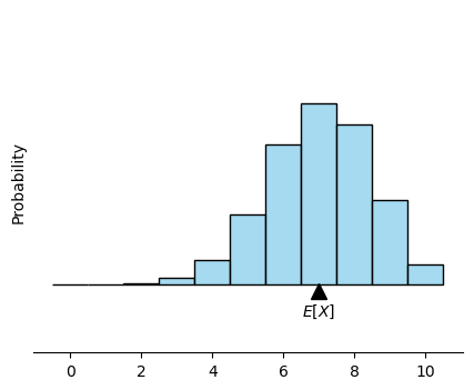
Drawing the histogram of a binomial distribution:

# import the necessary packages to compute and visualize in python
import numpy as np
import matplotlib.pyplot as plt
import seaborn as sns

# parameters for the binomial distribution
n = 10
p = 0.7

# generate binomial distribution
data = np.random.binomial(n, p, 10000)

# plot histogram using seaborn
plt.figure(figsize=(5, 4))
sns.histplot(data, 
             bins=np.arange(-0.5, n+1.5, 1), 
             kde=False, stat='probability', 
             color='skyblue', 
             edgecolor='black')

# calculate expected value E[X] = np
expected_value = n * p

# add a triangle and label it by E[X]
plt.plot(expected_value, -0.01, marker='^', markersize=10, color='black')
plt.text(expected_value, -0.04, '$E[X]$', ha='center', va='center')

# cleaning the graph, we don't need the numbers
plt.ylim(-0.1, 0.4)  
plt.tick_params(left=False, bottom=True, labelleft=False, labelbottom=True)
sns.despine(left=True, bottom=False)


plt.show()

/Users/boraferlengez/anaconda3/envs/bayes/lib/python3.11/site-packages/seaborn/_oldcore.py:1498: FutureWarning: is_categorical_dtype is deprecated and will be removed in a future version. Use isinstance(dtype, CategoricalDtype) instead
  if pd.api.types.is_categorical_dtype(vector):
/Users/boraferlengez/anaconda3/envs/bayes/lib/python3.11/site-packages/seaborn/_oldcore.py:1119: FutureWarning: use_inf_as_na option is deprecated and will be removed in a future version. Convert inf values to NaN before operating instead.
  with pd.option_context('mode.use_inf_as_na', True):

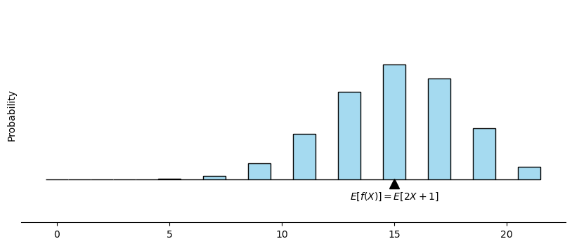
How to visualize the expectation of a function

# import the necessary packages to compute and visualize in python
import numpy as np
import matplotlib.pyplot as plt
import seaborn as sns

# parameters for the binomial distribution
n = 10
p = 0.7

# generate binomial distribution
data = 2*np.random.binomial(n, p, 10000)+1

# plot histogram using seaborn
plt.figure(figsize=(10, 4))
sns.histplot(data, 
             bins=np.arange(-0.5, 2*n+2.5, 1), 
             kde=False, stat='probability', 
             color='skyblue', 
             edgecolor='black')

# calculate expected value E[X] = np
expected_value = 2*n * p+1

# add a triangle and label it by E[X]
plt.plot(expected_value, -0.01, marker='^', markersize=10, color='black')
plt.text(expected_value, -0.04, '$E[f(X)] = E[2X+1]$', ha='center', va='center')

# cleaning the graph, we don't need the numbers
plt.ylim(-0.1, 0.4)  
plt.tick_params(left=False, bottom=True, labelleft=False, labelbottom=True)
sns.despine(left=True, bottom=False)

plt.show()

/Users/boraferlengez/anaconda3/envs/bayes/lib/python3.11/site-packages/seaborn/_oldcore.py:1498: FutureWarning: is_categorical_dtype is deprecated and will be removed in a future version. Use isinstance(dtype, CategoricalDtype) instead
  if pd.api.types.is_categorical_dtype(vector):
/Users/boraferlengez/anaconda3/envs/bayes/lib/python3.11/site-packages/seaborn/_oldcore.py:1119: FutureWarning: use_inf_as_na option is deprecated and will be removed in a future version. Convert inf values to NaN before operating instead.
  with pd.option_context('mode.use_inf_as_na', True):

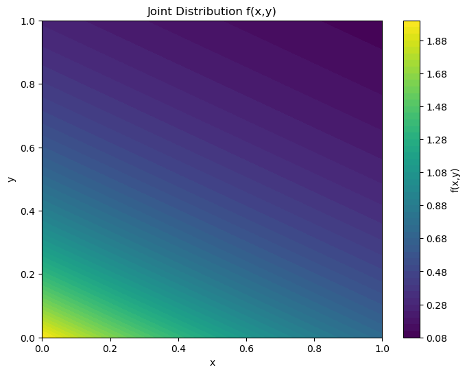
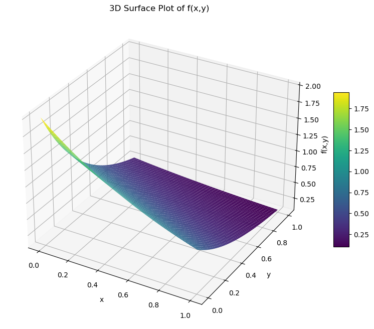
How to visualize a joint probability distribution of continuous random variables

def joint_distribution(x, y):
    return 2 * np.exp(-x) * np.exp(-2 * y)
x = np.linspace(0, 1, 400)
y = np.linspace(0, 1, 400)
X, Y = np.meshgrid(x, y)
Z = joint_distribution(X, Y)

plt.figure(figsize=(8, 6))
plt.contourf(X, Y, Z, 50, cmap='viridis')  # 50 is the number of contour levels
plt.colorbar(label='f(x,y)')
plt.title('Joint Distribution f(x,y)')
plt.xlabel('x')
plt.ylabel('y')
plt.show()

import matplotlib.gridspec as gridspec

def joint_distribution(x, y):
    return 2 * np.exp(-x) * np.exp(-2 * y)

x = np.linspace(0, 1, 400)
y = np.linspace(0, 1, 400)
X, Y = np.meshgrid(x, y)
Z = joint_distribution(X, Y)
# Marginal distribution of X (integrate out Y)
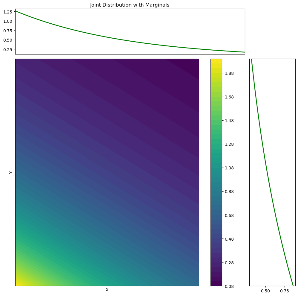
marginal_x = np.trapz(Z, y, axis=1)

# Marginal distribution of Y (integrate out X)
marginal_y = np.trapz(Z, x, axis=0)
# Set up the figure and gridspec
fig = plt.figure(figsize=(10, 10))
gs = gridspec.GridSpec(2, 2, width_ratios=[5, 1], height_ratios=[1, 5])
ax_joint = fig.add_subplot(gs[1, 0])
ax_marg_x = fig.add_subplot(gs[0, 0], sharex=ax_joint)
ax_marg_y = fig.add_subplot(gs[1, 1], sharey=ax_joint)

# Plot the joint distribution
c = ax_joint.contourf(X, Y, Z, 50, cmap='viridis')
fig.colorbar(c, ax=ax_joint)

# Plot the marginals
ax_marg_x.plot(x, marginal_x, 'g', lw=2)
ax_marg_y.plot(marginal_y, y, 'g', lw=2)

# Remove ticks from the marginals
ax_marg_x.set_xticks([])
ax_marg_y.set_yticks([])

# Set labels
ax_joint.set_xlabel('X')
ax_joint.set_ylabel('Y')
ax_marg_x.set_title('Joint Distribution with Marginals')

plt.tight_layout()
plt.show()

from mpl_toolkits.mplot3d import Axes3D

fig = plt.figure(figsize=(10, 8))
ax = fig.add_subplot(111, projection='3d')
surf = ax.plot_surface(X, Y, Z, cmap='viridis', edgecolor='none')
ax.set_title('3D Surface Plot of f(x,y)')
ax.set_xlabel('x')
ax.set_ylabel('y')
ax.set_zlabel('f(x,y)')
fig.colorbar(surf, ax=ax, shrink=0.5, aspect=10)
plt.show()

Homework 2, problem 1

You can copy and paste the following code in Google Colab to produce an interactive widget and see how the probability mass functions of \(X_n\) change for different values of \(\lambda\) or as \(n\) increases.
(Github pages only offer a static webpage, so the sliders won’t work here.)

import numpy as np
import matplotlib.pyplot as plt
import ipywidgets as widgets
from IPython.display import display

def probability(k, lambda_, n):
    """
    Compute the probability P(X=k/n) for given k, lambda, and n.
    """
    numerator = 1 - np.exp(-lambda_/n)
    denominator = np.exp(k*lambda_/n)
    return numerator / denominator

def plot_distribution(lambda_=2, n=10):
    k_values = np.arange(0, 5*n)  

    # Compute probabilities for each k
    probabilities = [probability(k, lambda_, n) for k in k_values]

    # Plot
    plt.figure(figsize=(10,6))
    plt.bar(k_values/n, probabilities, width=0.05)
    plt.xlabel('X = k/n')
    plt.ylabel('Probability')
    plt.title(f'Probability Distribution for λ = {lambda_} and n = {n}')
    plt.ylim(0, max(probabilities) + 0.05)  # Adjust y-axis limit for better visualization
    plt.show()

# Create interactive sliders
lambda_slider = widgets.FloatSlider(value=2, min=0.1, max=10, step=0.1, description='λ:')
n_slider = widgets.IntSlider(value=10, min=1, max=100, step=1, description='n:')

widgets.interactive(plot_distribution, lambda_=lambda_slider, n=n_slider)

---------------------------------------------------------------------------
ModuleNotFoundError                       Traceback (most recent call last)
Cell In[6], line 3
      1 import numpy as np
      2 import matplotlib.pyplot as plt
----> 3 import ipywidgets as widgets
      4 from IPython.display import display
      6 def probability(k, lambda_, n):

ModuleNotFoundError: No module named 'ipywidgets'

I was playing below with how the probabilities for \(X_n\) and for \(\lambda e^{-\lambda x}\):

import numpy as np
# for integrating we need the scipy package, that will allow us to run numerical computations in python such as numerical integration
from scipy.integrate import quad

def probability(k, lambda_, n): # lambda is used in python, hence i named the my parameter lambda_
    """
    Compute the probability P(X=k/n) for given k, lambda, and n.
    """
    numerator = 1 - np.exp(-lambda_/n)
    denominator = np.exp(k*lambda_/n)
    return numerator / denominator

def f(x, lambda_):
    """
    Define the probability density function of the exponential distribution
    """
    return lambda_ * np.exp(-lambda_ * x)


n = 5 # even for very small n, the values are very close
lambda_ = 0.5
k_values = np.arange(0, 100*n)

a = 1
b = 4

discrete_prob = sum([probability(k, lambda_, n) for k in k_values[a*n:b*n]])

exponential_prob = quad(f, a, b, args=(lambda_,))[0] # quad is the scipy function i used for the numerical integration of the exponential distribution
                                                    # quad gives two outputs: the numerical integral and an error estimate
                                                    # by putting [1] after the quad function, i'm grabbing the first output, namely the integral value

print(f'The integral of the probabily mass function of X_n for n={n} and lambda={lambda_} from a={a} to b={b}: {discrete_prob}')
print(f'The integral of the probabily density function of the exponential random variable for lambda={lambda_} from a={a} to b={b}: {exponential_prob}')

The integral of the probabily mass function of X_n for n=5 and lambda=0.5 from a=1 to b=4: 0.471195376476021
The integral of the probabily density function of the exponential random variable for lambda=0.5 from a=1 to b=4: 0.4711953764760207

Homework 2, problem 2

How to do symbolic integration in Python:

from sympy import symbols, integrate, exp

# define the symbols
x, lambda_ = symbols('x lambda_')

# define the function
f = lambda_ * exp(-lambda_ * x)

# find the antiderivative (indefinite integral) of the function
antiderivative = integrate(f, lambda_)

print(f"Antiderivative: {antiderivative}")

Antiderivative: Piecewise(((-lambda_*x - 1)*exp(-lambda_*x)/x**2, Ne(x**2, 0)), (lambda_**2/2, True))

The result in more human writing is:
The \(\displaystyle \int \lambda e^{\lambda x}d\lambda = (-\lambda x - 1)\frac{e^{\lambda x}}{x^2}\), if \(x\neq 0\). (otherwise the integral is \(\frac{\lambda^2}{2}\))