Random Variables (Discrete)

You can define a random variable \(X\) to be a function from a sample space \(\Omega\) to the reals \(\mathbb{R}\).

Note

Remark One way to think of a random variable is to think of the preimages of \(X\) (namely the outcomes that are assigned to the same number) They are events. So, effectively, when defining a random variable, we’re giving the same value to the outcomes that we want them to grouped together. That way, different events correspond to different values of the random variable.

We tend to classify random variables in two classes: Discrete and Continuous.

What matters is that if we have a discrete random variable, we can count things (things may be infinite, but still listable), as there is a jump between each possible value of the random variable, and addition is the usual summation:

\(\{5\leq X<8\} = \{X=5.5\} \cup \{X=6.3\} \cup \{X=7.9\}\)

When we have a continuous variable, we describe them mostly in terms of intervals and we trace outcomes in an event rather than counting the outcomes one by one. For most of the continuous random variables, we’ll be able to use techniques of calculus. For example, addition becomes definite integrals.

Baby example

Toss a coin twice and label the outcomes by the number of heads.
Then our random variable \(X\) takes the possible values \(\{0,1,2\}\), where

\(X=k\)	event
\(X=0\)	\(\{TT\}\)
\(X=1\)	\(\{HT,TH\}\)
\(X=2\)	\(\{HH\}\)

Then probabilities can be assigned to those events. A probability distribution is a function that assigns a probabilities to events. In the context of discrete random variables, we call the probability distributions as probability mass functions and in the context of continuous random variables, we call the probability distributions as probability density functions.

Back to baby example

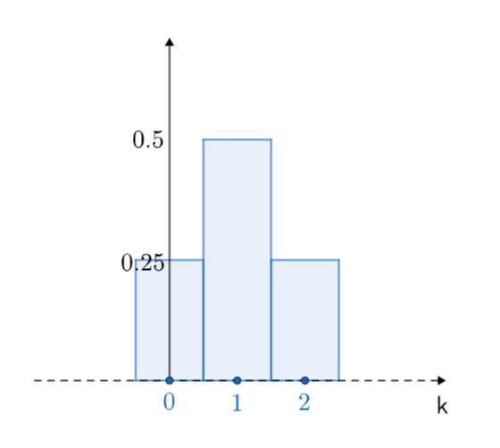
If a coin is assumed to be fair, then the probability mass function for the variable \(X\) we defined above can be written as

\(P(X=0)=\frac{1}{4}\), \(P(X=1)=\frac{1}{2}\) and \(P(X=2)=\frac{1}{4}\)

Remark

I think it’s important to have a temporal/causal hieararchy:

• “the chance experiment” comes before “knowing all possible outcomes”,

• “knowing all possible outcomes” comes before “grouping some outcomes and defining events”,

• “defining events” comes before “using numerical values as labels of events, i.e. defining a random variable”,

• “defining a random variable” comes before “assigning probabilities”

We can use histograms to represent probability mass functions visually.
The histogram for our baby example looks like:

(Popular) Discrete Random Variables

You can find a quite comprehensive list of random variables and their probability distributions (both discrete and continuous) on this nice wikipedia page: wiki:List_of_probability_distributions.
A probability distribution is

We’ll be interested in a few common discrete random variables so that we can use them in future examples:

Name	Experiment	Random variable	\(P(X=k)\)
Uniform	Pick a random number from among \(\{1,2,3,\dots,n\}\)	\(X=\textrm{Unif}(n)\) the number you picked	\(P(X=k)=\frac{1}{n}\) for \(k=1,2,\dots,n\)
Bernoulli trial	Toss a coin.	\(X=\textrm{Bern}(p)=1\), for heads and \(X=\textrm{Bern}(p)=0\) for tails.	\(P(X=1)=p\), \(P(X=0)=(1-p)\) for \(k=0\) or \(1\).
Binomial random variable	Repeat a Bernoulli trial \(n\) times.	\(X=\textrm{Bin}(n,p)=\) the number of heads you observe	\(P(X=k)={n \choose k}p^k(1-p)^{n-k}\) for \(k=0,1,\dots,n\)
Geometric random variable	Repeat Bernoulli trials until you get a heads.	\(X=\textrm{Geom}(p)=\) number tosses you observe.	\(P(X=k)=(1-p)^{k-1}p\) for \(k=1,2,3,\dots\)
Poisson random variable	Consider a large number of Bernoulli trials, where the probability of success is relatively small such that the product \(np=\lambda\) is still a moderate number.	\(X=\textrm{Pois}(\lambda)=\) number of successes in those trials.	\(\displaystyle P(X=k)=\frac{e^{-\lambda}\lambda^k}{k!}\) for \(k=0,1,2,\dots\)

Remark

One important thing we can check to make sure the probability mass functions are defined correctly is they need to add up to the probability of the sample space, which equals to one:

• (Discrete) uniform distribution: \(\sum_{k=1}^n P(X=k)=\sum_{k=1}^n \frac{1}{n}=n\cdot \frac{1}{n}=1\).

• Bernoulli distribution: \(\sum_{k=0}^1 P(X=k) = p + (1-p) = 1\).

• Binomial distribution: \(\sum_{k=1}^n P(X=k) = \sum_{k=1}^n {n \choose k}p^k(1-p)^{n-k}=1\) (exc.)

• Geometric distribution: \(\sum_{k=1}^{\infty} P(X=k) = \sum_{k=1}^{\infty} (1-p)^{k-1}p = p\sum_{k=1}^{\infty} (1-p)^{k-1} = p\sum_{k=0}^{\infty}(1-p)^k=p\cdot \frac{1}{1-(1-p)}=1\) (some calc 2 is happening here!).

• Poisson distribution: \(\sum_{k=0}^{\infty}\frac{e^{-\lambda}\lambda^k}{k!}=e^{-\lambda}\sum_{k=0}^{\infty}\frac{\lambda^k}{k!}=e^{-\lambda}e^{\lambda}=1\), since the Taylor series of \(e^\lambda = \sum_{k=0}^{\infty}\frac{\lambda^k}{k!}\).

Once we have a random variable and its probability mass/density function, we can compute some scalars that summarize some important aspects of our random variable.
Two of them are then to be very significant: The expected value and the variance of the random variable.

Expected Value of a (Discrete) Random Variable

The expected value (or mean) of a random variable \(X\) is defined to be as a weighted sum.
Each possible value of the random variable gets to have its probability as its weight:

\[E[X] = \sum_{k} k\cdot P(X=k)\]

Back to baby example

If we have a fair coin (\(p=\frac{1}{2}\)), then the expected value of the variable \(X\) in our baby example becomes:

\[\begin{split} \begin{aligned} E[X] & = \sum_{k} k\cdot P(X=k) \\ & = 0\cdot P(X=0) + 1\cdot P(X=1) + 2\cdot P(X=2) \\ & = 0\cdot \frac{1}{4} + 1\cdot \frac{1}{2} + 2\cdot \frac{1}{4} \\ & = 1 \end{aligned}\end{split}\]

What this computation gives us is that if we toss a fair coin twice, we expect to see 1 heads on average.

Note

Remark The geometric interpretation of the expected value of a random variable is the following:
The expected value is a horizontal value on the histogram of a random variable such that the histogram stays on balance and won’t tilt (clockwise or counterclockwise) if you put a pivot right at \(E[X]\).

(General Culture: Moments of a distribution)

If you remember some basic physics of mechanics, you’d see that the computation of \(E[X]\) looks like a moment computation. Expected value is the first moment of a distribution. For more about moments of a distribution (optional for us): Moment. Also a quick remark, the zeroth moment is always 1 for a probability distribution, the second moment after centralizing is the variance etc.

Remark: Python

I will try to draw make the visualizations using Python (maybe later I can add the R versions, or even better, you can send the R versions in the Telegram group chat and we’d have better notes.)
You can find the Python codes here.

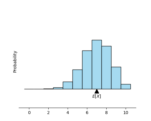
You can think of removing the locations of the horizontal values on a distribution via some other function \(f\).
For example \(f(k)=2k+1\) would move the original values of the random variable the following way: stretches away from horizontal middle by 2 and then shifts to right by 1.

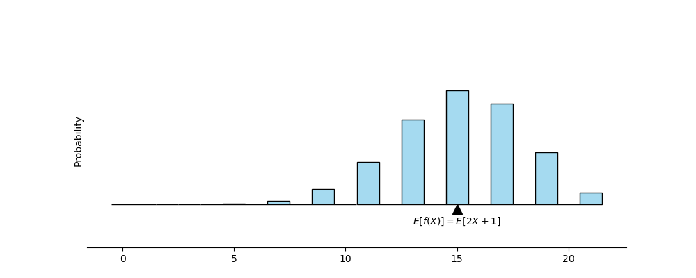
Note that all that happening is, the same events are now labeled by different numbers. The events stay the same, hence their probabilities stay the same. The only thing that changes is how we labeled them.
So, based on precalculus ideas, we have the following definition:

\[E[f(X)]=\sum_{k}f(k)\cdot P(X=k)\]

We call this the expected value of the function \(f\).

Hence using a geometric argument using the transformation of the horizontal axis, or using the algebraic definition of the expected value of a function, we can easily prove the following property:

\[E[aX+bY]=aE[X]+bE[Y]\]

However, expected values are not multiplicative, i.e. \(E[XY]\neq E[X]E[Y]\), unless the random variables \(X\) and \(Y\) are independent.

Two (discrete) random variables \(X\) and \(Y\) are independent if

\[P(X=k,Y=l)=P(X=k)\cdot P(Y=l)\]

for any \(k,l\), where \(P(X=k, Y=l)\) denotes the intersection event of the events \(X=k\) and \(Y=l\).

Another baby example

Toss a coin twice.

• Let \(X:=\) the number of heads (0, 1, or 2) in two tosses.
  Let \(Y=1\) if the second toss is heads, and zero otherwise.
  Then \(X\) and \(Y\) are dependent.

• Let \(X:=\) if the first toss is tails, and zero otherwise.
  Let \(Y=1\) if the second toss is heads, and zero otherwise.
  Then \(X\) and \(Y\) are independent.

If two random variables are independent, then we have: \(E[XY]=E[X]\cdot E[Y]\)

The difference \(E[XY]-E[X]E[Y]\) is called covariance of \(X\) and \(Y\), and the covariance of two independent random variables is zero if the variables are independent:

Proof

\[\begin{split} \begin{align*} E[XY] & =\sum_{k,l} k\cdot l\cdot P(XY=kl) \\ & \stackrel{\textrm{always}}{=}\sum_{k}\sum_{l} k\cdot l \cdot P(X=k,Y=l) \\ & \stackrel{\textrm{independence}}{=}\sum_{k}\sum_{l} k\cdot l\cdot P(X=k)P(Y=l) \\ & = \sum_{k}k\left(\sum_{l} l\cdot P(Y=l)\right)P(X=k) \\ & =\sum_{k}k\left(E[Y]\right)P(X=k) \\ & =E[Y]\sum_{k}k\cdot P(X=k), \textrm{ as $E[Y]$ is just a constant, and doesn't depend on $k$,} \\ & = E[Y]E[X] \end{align*} \end{split}\]

However, the converse is not true:
If \(Cov(X,Y)\stackrel{def}{=}E[XY]-E[X]E[Y]\), \(X\) and \(Y\) be still dependent.

Counterexample

Let \(P(X=1)=P(X=-1)=0.3\) and \(P(X=2)=P(X=-2)=0.2\). Note the since the probability mass function of \(X\) is symmetric, \(E[X]=0\) (exc.: or compute by hand).
Let \(Y=X^2\). Then \(E[Y]=1\cdot 0.6 + 4\cdot 0.4=2.2 >0\).
Note that \(X\) and \(Y\) are not independent random variables, as for example \(P(X=1,Y=1)=0.3 \neq 0.3 \cdot 0.6 = P(X=1)\cdot P(Y=1)\), as \(X=1\) is a subset of \(Y=1\).
However, \(E[XY]=E[X^3]=0=0\cdot 2.2 = E[X]E[Y]\), since \(X^3\) is again a symmetric discrete random variable (exc.: or compute by hand).

Conditional Expectance

Conditional expectance of a random variable \(X\) for a given value of another random variable \(Y\) is defined as follows:

\[E[X|Y=l]=\sum_{k} k\cdot P(X=k|Y=l)\]

A very useful property that follows is the law of total expectation (also called as Adam’s law):

\[ E[X]=E[E[X|Y]] \]

Proof

Let \(E[X|Y]=g(Y)\). Then we get
$\( \begin{align*} E[g(Y)] & = \sum_{l} g(l)\cdot P(Y=l) \\ & = \sum_{l}\left( \sum_{k}k\cdot P(X=k|Y=l)\right) P(Y=l)\\ & = \sum_{l}\sum_{k}k\cdot P(X=k|Y=l)P(Y=l)\\ & = \sum_{k}k\sum_{l}P(X=k,Y=l)\\ & = \sum_{k}k\cdot P(X=k) \\ & = E[X] \end{align*} \)$

Example (law of total expectation)

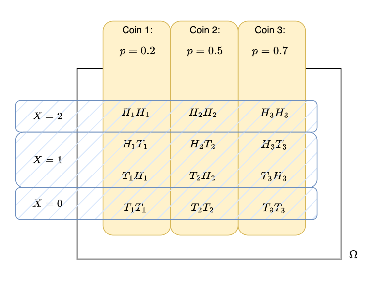
Assume we have three coins with probability of getting heads 0.2, 0.5 and 0.7, respectively.
The experiment consists of

• picking a coin with \(P(Y=1)=0.3\), \(P(Y=2)=0.5\), \(P(Y=3)=0.2\), where \(Y\) denotes the coin number,

• and tossing the coin twice.

Let \(X\) is defined to be the number of heads observed.

\[\begin{split} \begin{align*} E[X] & = E[E[X|Y=l]] \\ & = E[2p_i] \\ & = 0.3 \cdot (2\cdot 0.2) + 0.5 \cdot (2 \cdot 0.5) + 0.2\cdot (2\cdot 0.7) \\ & = 0.9 \end{align*} \end{split}\]

Expected Values of Popular Discrete Distributions

\(\textrm{Unif}(n)\)

\[E[\textrm{Unif}(n)]=\sum_{k=1}^n k\cdot P(\textrm{Unif}(n)=k)=\sum_{k=1}^n k\cdot \frac{1}{n} = \frac{1}{n}\sum_{k=1}^n k=\frac{1}{n}\cdot\frac{n(n+1)}{2}=\frac{n+1}{2}\]

\(\textrm{Bern}(p)\)

\[E[\textrm{Bern}(p)]=(1-p)\cdot 0 + 1\cdot p = p\]

\(\textrm{Bin}(n,p)\)

Let \(X_i\) be the Bernoulli random variable for the \(i^\textrm{th}\) trial.
Then we have \(\textrm{Ber}(n,p)=X_1 + X_2 + \dots + X_n\) (exc.).
Hence by linearity of expected values we have:

\[E[\textrm{Bin}(n,p)]=E[X_1 + X_2 + \dots + X_n]=E[X_1] + E[X_2] + \dots + E[X_n] = p + p + \dots + p = n\cdot p\]

\(\textrm{Geom}(p)\)

Let \(q=1-p\).

\[\begin{split} \begin{align*} E[\textrm{Geom}(p)] & = \sum_{k=1}^{\infty}k\cdot (1-p)^{k-1}p \\ & = \sum_{k=1}^{\infty}k\cdot (q)^{k-1}p \\ & = p\cdot \sum_{k=0}^{\infty} \frac{d}{dq}(q^k) \\ & = p\cdot \frac{d}{dq} \left( \sum_{k=0}^{\infty} q^k \right) \\ & = p\cdot \frac{d}{dq} \left( \frac{1}{1-q} \right) \\ & = \frac{p}{(1-q)^2} \\ & = \frac{1}{p} \end{align*} \end{split}\]

\(\textrm{Pois}(\lambda)\)

\[\begin{split} \begin{align*} E[\textrm{Pois}(\lambda)] & = \sum_{k=0}^{\infty} \frac{ke^{-\lambda}\lambda^k}{k!} \\ & = \lambda e^{-\lambda} \cdot \sum_{k=1}^{\infty} \frac{\lambda^{k-1}}{(k-1)!} \\ & \stackrel{i=k-1}{=} \lambda e^{-\lambda} \cdot \left( \sum_{i=0}^{\infty} \frac{\lambda^{i}}{i!} \right)\\ & = \lambda \cdot e^{-\lambda} \cdot e^{\lambda} \\ & = \lambda \end{align*} \end{split}\]

Variance of a (Discrete Random Variable)

The variance of a random variable \(X\) can be defined as \(Var(X)=Cov(X,X):=E[X^2]-\left( E[X]\right)^2\).

Another equivalent definition, and maybe a bit more fundamental, for \(Var(X)\) is \(Var(X)=\sigma_X^2 := E\left[\left(X-E[X]\right)^2\right]\).

We call the square-root of the variance of a random variable \(X\) as the standard deviation, denoted by \(\sigma_X\).

Equivalence of those two definitions:

\[\begin{split} \begin{align*} E\left[\left(X-E[X]\right)^2\right] & = \sum_{k} \left(k-E[X]\right)^2\cdot P(X=k) \\ & = \sum_{k} \left( k^2 - 2kE[X] + \left( E[X]\right)^2\right)\cdot P(X=k) \\ & = \sum_{k}k^2\cdot P(X=k) - 2E[X]\sum_{k}k\cdot P(X=k) + \left( E[X]\right)^2\sum_{k}P(X=k) \textrm{, where } E[X] \textrm{ is a constant that doesn't depend on } k,\\ & = E\left[X^2\right] - 2\left(E[X]\right)^2 + \left(E[X]\right)^2 \\ & = E\left[X^2\right] - \left(E[X]\right)^2 \end{align*} \end{split}\]

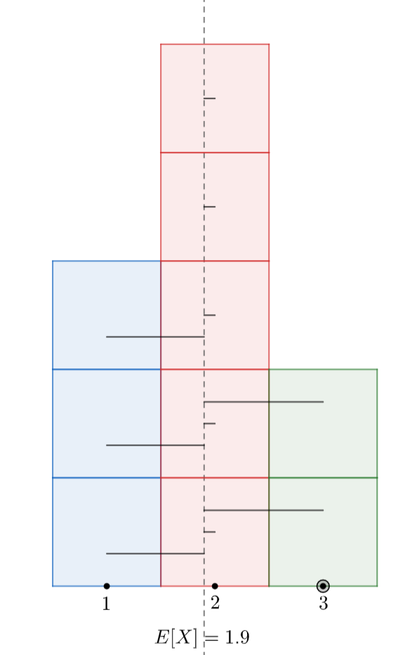
To understand the geometric intuition behind the variance, consider the following sample space, where each outcome is assumed to occur equally likely:

Advanced Remark

For those of you, that are familiar with some real analysis and linear algebra, random variables with mean zero form an inner product space (i.e. Hilbert space), where the covariance is the inner product and the standard deviation is the induced norm.

One good way to think of the standard deviation \(\sigma_X\) is the average of the errors from the mean.
Assume that we have a few equally likely outcomes in a sample space: \(\Omega = \{a_1, a_2, a_3, b_1, b_2, b_3, b_4, b_5, c_1, c_2\}\).
Define the discrete random variable \(X\) by:

\[\begin{split} X = \begin{cases} 1, & \textrm{if the outcome is } a_i \textrm{ for some } i=1,2,3\\ 2, & \textrm{if the outcome is } b_i \textrm{ for some } i=1,2,3,4,5\\ 3, & \textrm{if the outcome is } c_i \textrm{ for some } i=1,2 \end{cases} \end{split}\]

Then, the probabilities are given as

\[\begin{split} P(X=k) = \begin{cases} \frac{3}{10}, & \textrm{if } k=1 \\ \frac{5}{10}, & \textrm{if } k=2 \\ \frac{2}{10}, & \textrm{if } k=3 \end{cases} \end{split}\]

Hence \(E[X]=1\cdot 0.3 + 2\cdot 0.5 + 3\cdot 0.2 = 1.9\).
Moreover, \(E[X^2]=1\cdot 0.3 + 4\cdot 0.5 + 9\cdot 0.2 = 4.1\)
and therefore \(\sigma_X = \sqrt{Var(X)}=\sqrt{E[X^2] - (E[X])^2}=4.1 - 1.9^2 = 0.7\)

That value \(\sigma_X=0.7\) can be thought as (approximately) the average horizontal stick length in the following histogram:

Either using horizontal transformation of \(X\), or via the definition, we can show the following properties of the \(Var(X)\):

• \(Var(\textrm{constant})=0\)

• \(Var(aX +b)=a^2Var(X)\)

• \(Var(X+Y)=Var(X) + Var(Y) + 2Cov(X,Y)\)

Therefore, \(Var(X+Y)=Var(X)+Var(Y)\), if \(X\) and \(Y\) are independent random variables.
However, the converse is not true: see the example above.

Conditional Variance

Just like we defined conditional expectance, we can define the conditional variance of a random variable \(X\), given that another random variable \(Y=l\):

\[\begin{split} \begin{align*} Var(X|Y=l) & := E\left[ \left( E-E[X|Y=l]\right)^2 |Y=l\right] \\ & \stackrel{\textrm{exc.}}{=} E[X^2|Y=l] - (E[X|Y])^2 \end{align*} \end{split}\]

One can also show the following conditional variance formula:

\[Var(X)=E[Var(X|Y)]+Var[E[X|Y]]\]

I leave the following computations as exercise:

\(X\)	\(Var(X)\)
uniform	\(Var(\textrm{Unif}(n))=\frac{n^2 - 1}{12}\)
Bernoulli	\(Var(\textrm{Bern}(p))=p(1-p)\)
binomial	\(Var(\textrm{Bin}(n,p))=np(1-p)\)
geometric	\(Var(\textrm{Geom}(p))=\frac{1-p}{p^2}\)
Poisson	\(Var(\textrm{Pois}(\lambda))=\lambda\)