Hints for Homework 3

Hints for Homework 3#

Question 1#

Problem Suppose that our prior for \(\mu\) is \(\frac{2}{3} : \frac{1}{3}\) mixture of \(N(0,1)\) and \(N(1,1)\) and that a single observation is made \(x\sim N(\mu,1)\) and turns out to be equal to 2. What is the posterior probability that \(\mu>1\)?

One thing you need to remember is that when you have a mixture prior for a random variable, then its posterior is the mixture of the posteriors of the component densities. Namely, if
\(f(\mu) = \alpha g(\mu) + \beta h(\mu)\),
then
\(f(\mu | x) = \alpha(x) g(\mu |x) + \beta(x) h(\mu |x)\),
so this problem is about computing some pieces and putting them together.

If the prior follows a normal distribution, and the likelihood function is normal, then the posterior is normal:


prior	\(\displaystyle \mu \sim N(m_0,s_0^2)\)
prior density function	\(\displaystyle f(\mu)=\frac{1}{\sqrt{2\pi}s_0}e^{-\frac{(\mu - m_0)^2}{2s^2_0}}\)
likelihood	\(\displaystyle x\|\mu \sim N(\mu,\sigma^2)\)
likelihood density function	\(\displaystyle f(x\|\mu)=\frac{1}{\sqrt{2\pi}\sigma}e^{-\frac{(x - \mu)^2}{2\sigma^2}}\)
posterior	\(\displaystyle \mu\| x \sim N\left( \frac{m_0\cdot\sigma^2+x\cdot s^2_0}{\sigma^2 + s^2_0},\frac{\sigma^2 \cdot s^2_0}{\sigma^2+s^2_0}\right)\)
posterior density function	\(\displaystyle f(\mu\|x)= \frac{1}{\sqrt{2\pi}\left( \sqrt{\frac{\sigma^2 \cdot s^2_0}{\sigma^2+s^2_0}}\right)}\exp\left(-\frac{\left( \mu - \frac{m_0\cdot\sigma^2+x\cdot s^2_0}{\sigma^2 + s^2_0} \right)^2}{2 \cdot \frac{\sigma^2 \cdot s^2_0}{\sigma^2+s^2_0}}\right)\)

Find the posterior \(g(\mu |x=2)\) and \(h(\mu |x=2)\). Since \(x=2\) is given, all you need is to find 4 numbers:


prior	\(\displaystyle \mu \sim N(0,1^2)\)
likelihood	\(\displaystyle x\|\mu \sim N(\mu,1^2)\)
posterior	\(\mu \| x=2 \quad \sim \quad N(\boxed{?_1},\boxed{(?_2)^2})\)
posterior density function	\(\displaystyle g(\mu\| x=2)=\frac{1}{\sqrt{2\pi}\boxed{?_2}}e^{-\frac{\left(\mu - \boxed{?_1}\right)^2}{2\cdot \boxed{(?_2)^2}}}\)


prior	\(\displaystyle \mu \sim N(1,1^2)\)
likelihood	\(\displaystyle x\|\mu \sim N(\mu,1^2)\)
posterior	\(\mu \| x=2 \quad \sim \quad N(\boxed{?_3},\boxed{(?_4)^2})\)
posterior density function	\(\displaystyle h(\mu\| x=2)=\frac{1}{\sqrt{2\pi}\boxed{?_4}}e^{-\frac{\left(\mu - \boxed{?_3}\right)^2}{2\cdot \boxed{(?_4)^2}}}\)

Once you find \(g(\mu \|x=2)\) and \(h(\mu \|x=2)\), now you’ll need to find \(\alpha(2)\) and \(\beta(2)\), as

\(f(\mu | x=2) = \alpha(2) N(\boxed{?_1},\boxed{(?_2)^2}) + \beta(2) N(\boxed{?_3},\boxed{(?_4)^2})\)

While doing this part, you’ll need to use the following identities:

\(\alpha(2) + \beta(2) =1\)
\(\displaystyle \frac{\alpha(2)}{\beta(2)} = \frac{\alpha \int f(x|\mu)g(\mu)d\mu}{\beta \int f(x|\mu)h(\mu)d\mu}\), where \(\alpha = 2/3\) and \(\beta = 1/3\) are given.

My suggestion is to write \(f(x|\mu)g(\mu)\) (likelihood times prior \(g\)) and \(f(x|\mu)h(\mu)\) (likelihood times prior \(h\)) and compute their the integrals. The trick when computing the integrals you’ll most likely use is the following:

\(\displaystyle \int \frac{1}{\sqrt{2\pi}{\blacksquare}}e^{-\frac{\left( \mu - \bigstar\right)^2}{2\blacksquare^2}} d \mu =1\), no matter what the values of \(\blacksquare\) and \(\bigstar\) are.

So, when computing \(f(x|\mu)g(\mu)\) and \(f(x|\mu)h(\mu)\), combine the exponents, complete the square in the exponent of the form \((\mu - \bigstar)^2\) and the rest will be an expression in terms of \(x\), which you can take out of an integral that is computed with respect to \(d\mu\).

Question 2#

Problem Suppose that your prior beliefs about the probability \(p\) of success in Bernoulli trials have mean \(\frac{1}{3}\) and variance \(\frac{1}{32}\). Give a \(95\%\) posterior HDR for \(p\) given that you have observed 8 successes in 20 trials.

Remember that \(\displaystyle E[Beta(\alpha,\beta)]=\frac{\alpha}{\alpha+\beta}\) and \(\displaystyle Var(Beta(\alpha,\beta))=\frac{\alpha\beta}{(\alpha+\beta)^2(\alpha+\beta+1)}\).
So, you can figure out what \(\alpha\) and \(\beta\) are by solving the simpler equation \(\displaystyle E[Beta(\alpha,\beta)]=\frac{\alpha}{\alpha+\beta}=\frac{1}{3}\) first, writing \(\beta\) in terms of \(\alpha\) and then use \(\displaystyle Var(Beta(\alpha,\beta))=\frac{\alpha\beta}{(\alpha+\beta)^2(\alpha+\beta+1)}=\frac{1}{32}\).
Once you have \(\alpha\) and \(\beta\), you know the prior \(Beta(\alpha,\beta)\). We also know how to get the posterior using the binomial likelihood function: \(Beta\left(\alpha+\textrm{\# successes},\beta +\textrm{\# failures}\right)\).

To find the Highest Density Region (HDR), you can do the following (I’ll be using a random \(\alpha=5\) and \(\beta=10\) below).

Way 1: Use a Beta Distribution calculator you find online#

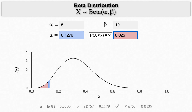
Find a Beta Distribution Calculator.
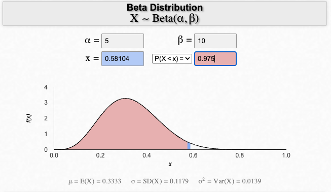
Find the \(x\) values by giving how much area you want to the left (or right) of a cut at \(x\) under the probability density function:

That gives the HDR \(=(0.13,0.58)\).

This method works well for unimodel symmetric distributions. If the model is not symmetric (like the one we have here), it gives a rough estimation.

Way 3: Run a Numerical Simulation using Python#

An easy way to find a highest density region is to run the following Python code in Google Colab (a numerical simulation):

Go to Google Colab.
Open a new notebook (you may need to log in using a gmail account).
Paste the following code: Use the \(\alpha\) and \(\beta\) you found earlier (I used a random \(\alpha=5\) and \(\beta=10\) in the example code).

import pymc as pm
import arviz as az
from scipy.stats import beta

# beta distribution parameters
alpha_param = 5
beta_param = 10

# generate samples for the simulation
samples = beta.rvs(alpha_param, beta_param, size=10000000)

# compute the HDI interval by counting samples
hdi_interval = az.hdi(samples, hdi_prob=0.95)

print("HDI Interval:", hdi_interval)

HDI Interval: [0.1137228  0.56301105]

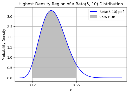
And here’s how to visualize it:

import numpy as np
import matplotlib.pyplot as plt
from scipy.stats import beta

# beta distribution parameters
alpha, beta_param = 5, 10

# define the beta distribution
dist = beta(alpha, beta_param)

# generate values from the beta distribution
x = np.linspace(0, 1, 1000)
pdf = dist.pdf(x)

# HDR boundaries (previously computed)
hdr_lower, hdr_upper = 0.12082921, 0.55393566

# plotting the probability density function
plt.figure(figsize=(6, 4))
plt.plot(x, pdf, label='Beta(5,10) pdf', color='blue')

# color and label the HDR
plt.fill_between(x, pdf, where=(x >= hdr_lower) & (x <= hdr_upper), color='gray', alpha=0.5, label='95% HDR')

# add ticks to denote the HDR interval endpoints on the horizontal axis
plt.xticks([hdr_lower, hdr_upper], [f'{hdr_lower:.2f}', f'{hdr_upper:.2f}'])

plt.title('Highest Density Region of a Beta(5, 10) Distribution')
plt.xlabel('x')
plt.ylabel('Probability Density')
plt.legend()
plt.grid(True)
plt.show()

_images/ef306e7b47a9dd00277dbe8b44bcd531c0b7ccb44e0658ae79b16ce515186d7d.png

Question 3#

Problem Suppose that you have a prior distribution for the probability \(p\) of success in a certain kind of gambling game which has mean 0.4, and that you regard your prior information as equivalent to 12 trials. You then play the game 25 times and win 12 times. What is your posterior distribution for \(p\)?

This question is very similar to question 2. Instead of using \(\displaystyle E[Beta(\alpha,\beta)]=\frac{\alpha}{\alpha+\beta}\) and \(\displaystyle Var(Beta(\alpha,\beta))=\frac{\alpha\beta}{(\alpha+\beta)^2(\alpha+\beta+1)}\), you will be using \(\displaystyle \alpha+ \beta = 12\) to find \(\alpha\) and \(\beta\) of the prior. Then you update the distribution using the binomial likelihood where \(\# \textrm{successes} = 12\), \(\# \textrm{failures} = 13\) (\(\textrm{total games} = 25\)).